Exponential Smoothing

Exponential Smoothing is a commonly used time series forecasting method for smoothing and predicting data. It assigns different weights to historical data, with more recent data receiving higher weights and older data receiving lower weights. SPSSAU offers three types of exponential smoothing: Simple Exponential Smoothing, Double Exponential Smoothing and Triple Exponential Smoothing. It is located in SPSSAU -> Comprehensive Evaluation -> Exponential Smoothing.

SPSSAU Operations

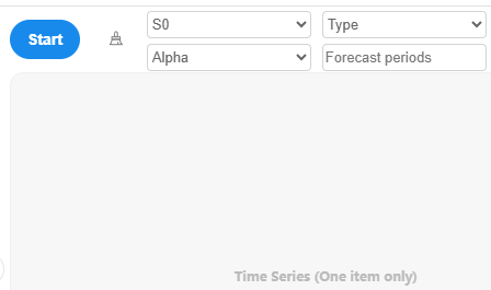
To perform the analysis, drag the time series data (only one item) into the right-hand box and click 'Start'. SPSSAU includes four parameters:

Initial Value (S0): Default is 'Auto', where the algorithm selects the optimal initial value based on the Root Mean Square Error (RMSE). Other options include the first period, the average of the first 2, 3, 4, or 5 periods.

Alpha: Default is 'Auto', where the algorithm selects the optimal alpha based on RMSE. Options range from 0.05 to 0.95 in increments of 0.05.

Smoothing Type: Default is 'Auto', where the algorithm selects the optimal type based on RMSE. Options include Simple, Double, and Triple Smoothing.

Backward Forecast Periods: Default provides forecasts for the next 12 periods, but users can customize this value.

SPSSAU Data Format

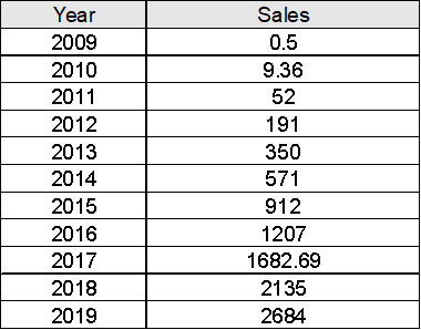
Exponential Smoothing is best suited for datasets with a small sample size. If the dataset includes a time term, it should be sorted sequentially but does not need to be included as an analysis item (it can be placed in the 'Label').

Algorithm

Simple Exponential Smoothing

Simple Exponential Smoothing is a basic time series forecasting method. The calculation steps are as follows:

1.Initialize the Smoothed Value

Choose the initial smoothed value S₁, typically the first observed value x₁：S₁ = x₁, which can be selected automatically by SPSSAU or manually.

2.Set the Smoothing Constant

The smoothing constant, α, ranges between 0 and 1. A larger α makes the model more sensitive to recent data.

3.Compute the Smoothed Value

For each time point t (t > 1), calculate S_t: S_t = αx_t + (1 - α)S_t-1.
x_t: actual value at time t.
S_t-1: smoothed value at time t - 1

4.Compute Forecast Values

For time t + 1, the forecast value {\hat{x}}_{t+1} is: $${\hat{x}}_{t+1}=S_t$$

5.Compute Forecast Errors

Forecast error e_t is defined as: $$e_t=x_t-{\hat{x}}_t$$ Absolute error (AE): $$\mathrm{A}\mathrm{E}=|x_t-{\hat{x}}_t|$$

6.Evaluate Forecast Accuracy

Forecast Accuracy is assessed using RMSE, MSE, MAE, or MAPE: $$\mathrm{R}\mathrm{M}\mathrm{S}\mathrm{E}=\sqrt{\frac{1}{n}\sum _{t=1}^n{e}_t^2}$$ $$\mathrm{M}\mathrm{S}\mathrm{E}=\frac{1}{n}\sum _{t=1}^n{e}_t^2$$ $$\mathrm{M}\mathrm{A}\mathrm{E}=\frac{1}{n}\sum _{t=1}^n\left|e_t\right|$$ $$\mathrm{M}\mathrm{A}\mathrm{P}\mathrm{E}=\frac{1}{n}\sum _{t=1}^n\left|\frac{e_t}{x_t}\right|$$

Double Exponential Smoothing

Double Exponential Smoothing is suitable for data with linear trends, such as per capita GDP.

1.Initialize the Smoothed Value

Choose the initial smoothed value S₁, typically the first observed value x₁：S₁ = x₁, which can be selected automatically by SPSSAU or manually.

2.Compute Smoothed Values

$$\{\begin{array}{c}{S}_t^{(1)}=\alpha x_t+(1-\alpha )S_{t-1}^{(1)}\\ S_t^{(2)}=\alpha S_t^{(1)}+(1-\alpha )S_{t-1}^{(2)}\end{array}$$ S_t^{(1)}: Simple Smoothing, S_t^{(2)}: Double Smoothing. x_t: actual value at time t, α: corrected error.

3.Compute Trend

When applying Double Exponential Smoothing to linear trend data, its essence is to identify a linear regression trend line. Mathematically, this can be represented by the following formula: {\hat{y}}_{t+T}=a_t+b_t\times T, where T represents the predicted value for the future period T, and a_t and b_t are the parameters of the linear regression trend line. These parameters are calculated using the following formulas: $$\{\begin{array}{c}{a}_t=2S_t^{(1)}-S_t^{(2)}\\ b_t=\frac{\alpha }{1-\alpha }(S_t^{(1)}-S_t^{(2)})\end{array}$$ Out-of-sample forecast values (prediction values) are computed using: $${\hat{y}}_{t+T}=a_t+b_t\times T,T=1,2,\cdots$$ In-sample forecast values (fitted values) are computed as: $${\hat{y}}_{t+1}=a_t+b_t$$

4.Compute Forecast Errors

The forecast error e_t is defined as the difference between the actual value and the predicted value: $$e_t=x_t-\widehat{x_t}$$ The absolute error (AE) is calculated as: $$\mathrm{A}\mathrm{E}=|x_t-\widehat{x_t}|$$

5.Assess Forecast Accuracy

Forecast accuracy can be evaluated using RMSE, MSE, MAE, or MAPE: $$\mathrm{R}\mathrm{M}\mathrm{S}\mathrm{E}=\sqrt{\frac{1}{n}\sum _{t=1}^n{e}_t^2}$$ $$\mathrm{M}\mathrm{S}\mathrm{E}=\frac{1}{n}\sum _{t=1}^n{e}_t^2$$ $$\mathrm{M}\mathrm{A}\mathrm{E}=\frac{1}{n}\sum _{t=1}^n\left|e_t\right|$$ $$\mathrm{M}\mathrm{A}\mathrm{P}\mathrm{E}=\frac{1}{n}\sum _{t=1}^n\left|\frac{e_t}{x_t}\right|$$ n: the number of forecast points, e_t: error.

Triple Exponential Smoothing

Triple Exponential Smoothing extends Double Exponential Smoothing by adding another level of smoothing, making it suitable for time series with a curvilinear growth trend, such as per capita GDP data. The calculation process is as follows:

1.Initialize Smoothing Values and Seasonal Index

Choose the initial smoothed value S₁, typically the first observed value x₁：S₁ = x₁, which can be selected automatically by SPSSAU or manually.

2.Compute Smoothing Formulas

$$\{\begin{array}{c}{S}_t^{(1)}=\alpha y_t+(1-\alpha )S_{t-1}^{(1)}\\ S_t^{(2)}=\alpha S_t^{(1)}+(1-\alpha )S_{t-1}^{(2)}\\ S_t^{(3)}=\alpha S_t^{(2)}+(1-\alpha )S_{t-1}^{(3)}\end{array}$$ S_t^{(1)}: Simple Smoothing, S_t^{(2)}: Double Smoothing. x_t: actual value at time t, α: corrected error.

3.Compute Trend

When applying Triple Exponential Smoothing to curvilinear trend data, it essentially finds a quadratic regression trend line. Mathematically, this is given by: $${\hat{y}}_{t+T}=a_t+b_t\times T+c_t\times T^2$$ a_t,b_t, and c_t are parameters of the quadratic trend line, computed as: $$\{\begin{array}{c}{a}_t=3S_t^{(1)}-3S_t^{(2)}+S_t^{(3)}\\ b_t=\frac{\alpha }{2(1-{\alpha }^2)}[(6-5\alpha )S_t^{(1)}-2(5-4\alpha )S_t^{(2)}+(4-3\alpha )S_t^{(3)}]\\ c_t=\frac{{\alpha }^2}{(1-\alpha {)}^2}[S_t^{(1)}-2S_t^{(2)}+S_t^{(3)}]\end{array}$$ Out-of-sample forecast values (prediction values): $${\hat{y}}_{t+T}=a_t+b_t\times T+c_t\times T^2,T=1,2,\cdots$$ In-sample forecast values (fitted values): $${\hat{y}}_{t+1}=a_t+b_t+c_t$$

4.Compute Forecast Errors

The forecast error e_t is defined as the difference between the actual value and the predicted value: $$e_t=x_t-{\hat{x}}_t$$ The absolute error (AE) is calculated as: $$\mathrm{A}\mathrm{E}=|x_t-{\hat{x}}_t|$$

5.Assess Forecast Accuracy

Forecast accuracy can be evaluated using RMSE, MSE, MAE, or MAPE: $$\mathrm{R}\mathrm{M}\mathrm{S}\mathrm{E}=\sqrt{\frac{1}{n}\sum _{t=1}^n{e}_t^2}$$ $$\mathrm{M}\mathrm{S}\mathrm{E}=\frac{1}{n}\sum _{t=1}^n{e}_t^2$$ $$\mathrm{M}\mathrm{A}\mathrm{E}=\frac{1}{n}\sum _{t=1}^n\left|e_t\right|$$ $$\mathrm{M}\mathrm{A}\mathrm{P}\mathrm{E}=\frac{1}{n}\sum _{t=1}^n\left|\frac{e_t}{x_t}\right|$$ n: the number of forecast points, e_t: error.

References

【1】The SPSSAU project (2024). SPSSAU. (Version 24.0) [Online Application Software]. Retrieved from https://www.spssau.com.
【2】周俊,马世澎. SPSSAU科研数据分析方法与应用.第1版[M]. 电子工业出版社,2024.