Outlier
If outliers are detected during analysis, you can configure and process them via [Data Processing] → [Outlier]. Outlier Settings consist of two components: 'Judgment Standard' and 'Outlier Handling', as shown in the table below.
| Item | Description |
|---|---|
| Judgment Standard | Define the standard for identifying outliers, e.g., height greater than 2.2 meters. |
| Outlier Handling | Apply corresponding handling to detected outliers. |
Judgment Standard
When setting judgment standard, for example, if analysis reveals that heights above 2.2 meters are outliers, you can set 'Number > 2.2' as the standard. Standard settings also include 'Missing Values,' which refer to null values in the raw data. Other available criteria include: equal to a specific number, less than a specific number, or deviation from the standard deviation range (typically 2 or 3 times the standard deviation, see Section 2.2.3 for details). There are five different standards in total. If any selected standard is met, the data point will be considered an outlier.
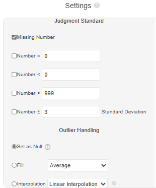
Outlier Handling
After defining judgment standard, you need to specify how the detected outliers should be handled. There are three mutually exclusive processing methods: 'Set to Null', 'Imputation', and 'Interpolation.'
| Handling | Description |
|---|---|
| Set to Null | Replace detected outliers with Null. |
| Imputation | Including six methods: mean, median, mode, random value, zero, or custom value. |
| Interpolation | Including linear interpolation and 'linear trend interpolation.' |
'Set to Null' is the most commonly used method, directly setting outliers to Null. However, this may reduce the valid sample size, so it is recommended for datasets with a large sample size.
Imputation includes six methods. mean, median, or mode imputation replaces outliers with the mean, median, or mode of the remaining data points. Random value imputation replaces outliers with a randomly generated number. 'Zero' imputation replaces outliers with the number 0. Custom value imputation replaces outliers with 'a user-defined number.'
Interpolation includes two approaches: linear interpolation and 'linear trend interpolation.'
| ID | Original Data | Linear Interpolation | Linear Trend Interpolation |
|---|---|---|---|
| 1 | 1 | 1 | 1 |
| 2 | 3 | 3 | 3 |
| 3 | 4 | 4 | 4 |
| 4 | Outlier | 5 | 5.46511 |
| 5 | 6 | 6 | 6 |
| 6 | 9 | 9 | 9 |
Linear interpolation estimates outlier values using the nearest previous and next data points. For example, in the table above, ID 4 is an outlier. The closest data points are: ID 3: (3,4) and ID 5: (5,6). Drawing a straight line between these two points gives the equation: y=x + 1. Substituting x = 4 (the ID of the outlier), we get: y = 4 + 1 = 5. Thus, the linear interpolation value for the outlier is 5. ID represents the sequence number of the original data. If there are 100 samples, ID will range from 1 to 100.
'Linear trend interpolation' uses linear regression to fit a trend based on the non-outlier data (X represents ID numbers and Y represents original data). A linear regression equation is calculated using all non-outlier values (see Chapter 5 for more on linear regression). For the dataset above, the regression equation is: Y = −0.30233 + 1.44186 × X. Substituting X = 4 (the ID of the outlier), we get: Y = −0.30233 + 1.44186 × 4 = 5.46511. Thus, the 'linear trend interpolation' for the outlier is 5.46511.