Grey Relational Analysis

Grey Relational Analysis is a quantitative method for analyzing and evaluating relationships between different factors. It is widely used in economics, management, and engineering. The principle is to assess the similarity in geometric shape between the reference sequence (mother sequence) and the comparative sequence (feature sequence). It is located in SPSSAU -> Comprehensive Evaluation -> Grey Relational Analysis.

SPSSAU Operations

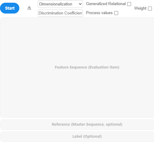
Drag the feature sequence and mother sequence into the right-hand box and click 'Start'. If there is a label item, it can also be dragged into the corresponding box. SPSSAU involves five parameters:

Dimensionalization: SPSSAU provides two methods: Mean Centering and Initialization. By default, no dimensionalization is applied.

Discrimination Coefficient: Default value is 0.5; users can input their own value.

Generalized Relational: Default is unselected; if selected, generalized relational results are output.

Indicator Weight: If feature sequences have their own weights, this option allows users to set them. Default is unselected, meaning all weights are 1.

Save Process Values: If selected, grey relational coefficients will be saved as new titles, similar to "Grey_****_****".

SPSSAU Data Format

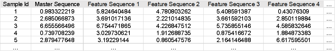
Grey relational analysis studies the degree of association between data, specifically the relationship between characteristic sequences and the reference sequence. The reference sequence is uniquely identified by a single column, while each characteristic sequence is represented by one column. The sample numbers in the figure serve only as identifiers and have no actual significance in the analysis. They are used to label the sample IDs and do not need to be utilized during the analysis. However, they can be dragged into the 'Label' field if desired.

Algorithm

1.Determine Sequence Data

First, identify the data to be analyzed, including the reference sequence and feature sequences.

2.Data Scaling

Perform scaling on the original data to eliminate the influence of dimensions. SPSSAU provides two scaling methods: Mean Centering and Initialization.

The formula for Mean Centering is:

$$\frac{x}{\overline{x}}$$

\overline{x} represents the mean. In the formula, the numerator is X, while the denominator is the mean of X. The resulting value indicates the multiple of the mean. Mean Centering is typically applied only to datasets where all values are greater than zero.

The formula for Initialization is:

Initialization: \frac{x}{x_0}, x₀ represents initial value.

In Initialization, the denominator x₀ is the first value of the original dataset. This method is commonly used in scenarios such as comparing GDP values over time, where all subsequent values are expressed as multiples of the GDP in a reference year (e.g., the year 2000). Initial value scaling is typically applied only to datasets where all values are greater than zero.

3.Calculate Grey Relational Coefficients

First, compute the absolute differences between each feature sequence and the reference sequence using the following formula:

$${△}_{ij}=|x_i^{\prime }-x_j^{\prime }|$$

Calculate the relational degree between the reference sequence and feature sequences:

$${\xi }_{ij}=\frac{{△}_{min}+\rho {△}_{max}}{{△}_{ij}+\rho {△}_{max}}$$

• ξ_ij represents the grey relational coefficient between the reference sequence and the feature sequence.
• Δ_ij represents the difference between the reference and feature sequences.
• Δ_min is the minimum of all differences.
• Δ_max is the maximum of all differences.
• ρ is the discrimination coefficient, typically ranging between [0,1], with a default value of 0.5, but it can be adjusted in SPSSAU.

4.Calculate Grey Relational Degree

For each feature sequence, calculate the average relational degree with the reference sequence:

$$\overline{{\xi }_j}=\frac{1}{n}\sum _{i=1}^n{\xi }_{ij}\times W_j$$

n represents the number of feature sequences. W_j represents the assigned weight, which defaults to 1. If customized weights are assigned, SPSSAU will first normalize them before applying the calculation.

5.Rank

Rank the feature sequences based on \overline{{\xi }_j}. A higher value indicates a stronger relation.

Generalized Relational Degree

1.Absolute Relational Degree

Step 1: Initial Zeroization

Initial zeroization involves subtracting the first value from each sequence. This step is performed for dimensional processing so that the first-row values all become zero.

Step 2: Calculate s₀ and s₁

Calculate s₀ and s₁ using the following formula:

$$s_0=\sum _{k=1}^{n-1}x(k)+\frac{1}{2}x(n)$$ $$s_1=\sum _{k=1}^{n-1}x(k)+\frac{1}{2}x(n)$$

n represents the sample size. This formula sums the first n-1 numbers and adds half of the last value.

Step 3: Calculate Absolute Relational Degree

Absolute relational degree is then calculated using:

\xi (k)=\frac{1+\left|s_0\right|+\left|s_1\right|}{1+\left|s_0\right|+\left|s_1\right|+|s_1-s_0|}, k is sample ID

2.Relative Relational Degree

Step 1: Initialization

Step 2: Initial Zeroization

Step 3: Calculate s₀ and s₁

Step 4: Calculate Absolute Relational Degree

The only difference between relative and absolute relational degree calculations is that relative relational degree starts with initialization, where each sequence is divided by its first value for dimensional processing. Steps 2, 3, and 4 remain identical to absolute relational degree calculations.

3.Comprehensive Relational Degree

After obtaining both absolute and relative relational degrees, they can be combined using weighted aggregation:

Comprehensive Relational Degree = ρ × Absolute Relational Degree + (1 - ρ) × Relative Relational Degree, where ρ represents weight coefficient with a default value of 0.5.

The comprehensive relational degree is the weighted calculation of the absolute and relative relational degrees. Typically, the weight coefficient for the absolute association degree is set to 0.5, but this value can be adjusted and recalculated as needed.

References

【1】The SPSSAU project (2024). SPSSAU. (Version 24.0) [Online Application Software]. Retrieved from https://www.spssau.com.
【2】周俊,马世澎. SPSSAU科研数据分析方法与应用.第1版[M]. 电子工业出版社,2024.
【3】郭秀云. 灰色关联法在区域竞争力评价中的应用[J]. 统计与决策, 2004(11):55-56.
【4】灰色关联法和层次分析法在盆栽多头小菊株系选择中的应用[J]. 中国农业科学, 2012, 45(17):3653-3660.