Grey Prediction Model

Grey Prediction Model is a forecasting method based on grey system theory, suitable for handling small samples and uncertainty problems. It is located in SPSSAU -> Comprehensive Evaluation -> Grey Prediction Model.

SPSSAU Operations

Drag the analysis item (only one item) into the right-hand box and click 'Start'. Additionally, during analysis, the research sequence name (i.e., label) can be dragged into the 'Label' box. SPSSAU involves three parameters: Model, Shift Transformation, and Backward Prediction Periods.

Model: The default is GM(1,1).

Shift Transformation: This parameter is selected by default. Data usually need to pass the level ratio test. If they do not, SPSSAU will automatically add a constant value c to ensure the data meet the requirement before conducting grey prediction analysis.

Backward Prediction Periods: By default, it provides predictions for 12 backward periods, but users can customize this setting.

SPSSAU Data Format

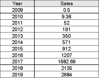
GM(1,1) Model is typically used for forecasting with very small sample sizes. If the data include a time variable, it does not need to be included in the analysis item (it can be placed in the 'Label' item). However, when organizing data, they should generally be sorted in chronological order before inputting.

Algorithm

1.Data Preparation

First, gather the time series data to be predicted, usually represented as an array:

X = (x₁,x₂,...x_n)

x₁ is the initial value, and x₂,...,x_n are subsequent observations.

2.Shift Transformation

If 'Shift Transformation' is selected, the system first conducts the level ratio test using the formula:

$$\lambda =\frac{x_{i-1}}{x_{{}_i}}$$

The values must fall within [e^-2/(n+1),e^2/(n+1)]. If not, SPSSAU will add a fixed number to the data sequence and then reapply the test. This fixed number is known as the shift transformation value. All subsequent calculations are based on the transformed data, but during final prediction, the shift value is subtracted.

3.Cumulative Generation Sequence (AGO)

AGO is performed to obtain a new sequence:

$$Y=(y_1,y_2,\dots ,y_n)$$ $$y_k=\sum _{i=1}^k{x}_i(k=0,1,2,\dots ,n)$$

4.Establish the Grey Model

Using the cumulative sequence, the grey model is constructed as follows:

$$\frac{dy}{dt}+ay=b$$

Discretization yields:

$$y_{k+1}-y_k+a{y}_k=b$$

5.Parameter Estimation

The model parameters a and b are estimated using the least squares method. Define:

$$\left[\begin{array}{c}{y}_1\\ y_2\\ ⋮\\ y_{n-1}\end{array}\right]=\left[\begin{array}{cc}-0.5(y_0+y_1)& 1\\ -0.5(y_1+y_2)& 1\\ ⋮& ⋮\\ -0.5(y_{n-2}+y_{n-1})& 1\end{array}\right]\left[\begin{array}{c}a\\ b\end{array}\right]$$

6.Prediction Calculation

Using the estimated parameters a and b, future predictions are calculated with the formula:

$${\hat{y}}_{k+1}=(y_1-\frac{b}{a})e^{-ak}+\frac{b}{a}$$

{\hat{y}}_{k+1}represents the predicted value at time k + 1.

7.Inverse Accumulation Generation

The predicted cumulative values are then converted back to original data scale:

$${\hat{x}}_{k+1}={\hat{y}}_{k+1}-{\hat{y}}_k$$

If shift transformation was applied, the shift value is subtracted:

$${\hat{x}}_{k+1}={\hat{y}}_{k+1}-{\hat{y}}_k-\mathrm{s}\mathrm{h}\mathrm{i}\mathrm{f}\mathrm{t}$$

8.Model Evaluation Metrics

SPSSAU provides various evaluation metrics, as shown below:

Model Fit Metrics
Evaluation Metric	Description
Residual	Difference between actual and predicted values; the smaller, the better.
Relative Error	Absolute residual divided by actual value; the smaller, the better.
Level Ratio Deviation	Model fitting bias; the smaller, the better.
Posterior Difference Ratio (C)	Precision test metric; calculated as residual variance / data variance; the smaller, the better.
Small Error Probability (p Value)	Indicator of prediction accuracy; the larger, the better.
RMSE (Root Mean Square Error)	Square root of the mean squared residual; the smaller, the better.

Residual

e=\hat{x}-x

Relative Error

{\epsilon }_i=\frac{|x_i-{\hat{x}}_i|}{x_i}\times 100\mathrm{\%}

Level Ratio Deviation

{\rho }_i=1-\frac{1-0.5a}{1+0.5a}\times \lambda, ρ_i represents level ratio deviation, a is development coefficient, and λ is level ratio.

Posterior Difference Ratio (C)

C=\frac{S_2}{S_1}, C represents level ratio deviation.

S₁ is sequence variance, calculated as: S_1=\frac{1}{n-1}\sum _{i=1}^n(x_i-\frac{1}{n}\sum _{i=1}^n{x}_i{)}^2

S₂ is residual variance, calculated as: S_2=\frac{1}{n-1}\sum _{i=1}^n(|x_i-\widehat{x_i}|-\frac{1}{n}\sum _{i=1}^n|x_i-\widehat{x_i}|{)}^2

Small Error Probability (p Value)

p=P|e_i-\overline{e}|\le 0.6745\times S_1,S₁ represents sequence variance.

\overline{e}=\frac{1}{n-1}\sum _{i=2}^n{e}_i, e_i represent residuals . The first value is not included in the calculation (as the residual is always zero at the first value).

RMSE (Root Mean Square Error)

RMSE=\sqrt{\frac{1}{n-1}\sum _{i=2}^n{e}_i^2}

References

【1】The SPSSAU project (2024). SPSSAU. (Version 24.0) [Online Application Software]. Retrieved from https://www.spssau.com.
【2】周俊,马世澎. SPSSAU科研数据分析方法与应用.第1版[M]. 电子工业出版社,2024.