List

Generate Variables

Generate Variables is commonly used during data cleaning. SPSSAU provides six categories of Generate Variables, including Common, Scaling, Scientific, Summarization, Date-Related, and Other. The steps are as follows:

Select 'Title' and use the ctrl or shift keys to select multiple titles for batch processing.

Set Options: Simply select 'Title', configure the settings on the right-hand panel, and click 'Confirm'.

Screenshot and summary of Generate Variables are as follows:

Item	Description
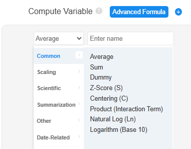
Common	8 features, including: Average, Sum, Dummy, Z-Score (S), Centering (C), Product (Interaction Term), Natural Log (Ln), and Logarithm (Base 10).
Scaling	15 features, including: Normalization, Mean Centering, Positive Transformation, Negative Transformation, Moderation, Intervalization, Initialization, Min Scaling, Max Scaling, Sum Normalization, Sum of Squares Normalization, Fixed Value, Offset Fixed, Close Interval, and Offset Interval.
Scientific	7 features, including: Square, Square Root, Absolute, Reciprocal, Opposite, Cube, and Round.
Summarization	4 features, including: Max, Min, Median, and Count.
Date-Related	5 features, including: Date Processing, Date Subtraction, Lag, Difference, and Seasonal Difference.
Other	10 features, including: Sample ID, Box-Cox, Rank, Winsorizing, Trimming, Johnson Transformation, Ranking, Divide, Subtract, and Non-negative Shift.

Common

X1	X2	Average	Sum	Product (Interaction Term)
1	2	1.5	3	2
2	3	2.5	5	6
3	4	3.5	7	12
3	5	4.0	8	15

For example, given variables X1 and X2, the Average and Sum of the two variables are calculated as shown in the 3rd and 4th columns, respectively. The Product (Interaction Term) of the selected variables is displayed in the 5th column. Additionally, Common includes Z-Score (S), Centering (R), Natural Log (Ln), and Logarithm (Base 10):

X1	Z-Score (S)	Centering (R)	Natural Log (Ln)	Logarithm (Base 10)
1	-1.3056	-1.2500	0	0
2	-0.2611	-0.2500	0.6931	0.3010
3	0.7833	0.7500	1.0986	0.4771
3	0.7833	0.7500	1.0986	0.4771

Z-Score (S) of X1 transforms the data to have a mean of 0 and a standard deviation of 1. The formula for Z-Score (S) is as follows.

Z - Score (S) = $\frac{x - \bar{x}}{S t d}$ , $\bar{x}$ represents the mean, Std represents the standard deviation

Centering (R) transforms the data to have a mean of 0, and the formula is as follows.

Centering(R) = x - $\bar{x}$ , $\bar{x}$ represents the mean

Typically, if the numbers are very large, you can use Natural Log (Ln) or Logarithm (Base 10) to compress the data.

Scaling

Scaling refers to compressing data within a specified range. Certain methods also unify the data's direction, such as converting a metric (e.g., default rate) where lower is better into a metric where higher is better. Scaling is a collective term for a series of processing methods. SPSSAU includes 15 items, as follows:

Item	Description	Note
Normalization	Scales values to [0,1].	N/A
Mean Centering	Values represent multiples of the mean.	Usually applies to positive values only.
Positive Transformation	Scales values to [0,1], where higher is better.	N/A
Negative Transformation	Scales values to [0,1], where lower is better.	N/A
Moderation	Higher values indicate closer proximity to a target.	N/A
Intervalization	Compresses values into a specified range.	N/A
Initialization	Values represent multiples of the initial value.	Applies to positive values only.
Min Scaling	Values represent multiples of the minimum value.	Applies to positive values only.
Max Scaling	Values represent multiples of the maximum value.	Applies to positive values only.
Sum Normalization	Values represent their proportion of the sum.	Applies to positive values only.
Sum of Squares Normalization	Values represents 'relative proportions.'	Applies to positive values only.
Fixed Value	The closer to a specific number, the better. After processing, values range between [0,1].	N/A
Offset Fixed	The farther from a specific number, the better. After processing, values range between [0,1].	N/A
Close Interval	The closer to a specific interval, the better. After processing, values range between [0,1].	N/A
Offset Interval	The farther from a specific interval, the better. After processing, values range between [0,1].	N/A

The formulas are as follows：

In Normalization, the numerator is the difference between x and x_Min, while the denominator is the difference between x_Max and x_Min, which remains constant. When the numerator reaches its maximum, it equals the denominator, resulting in a normalized value of 1. When the numerator is at its minimum (0), the normalized value is 0. Thus, after normalization, values are constrained within [0,1].

$N o r m a l i z a t i o n : \frac{x - x_{M i n}}{x_{M a x} - x_{M i n}}$

In Mean Centering, the numerator is x, and the denominator is the mean of x, representing the multiple of the mean. This method is generally applied when all values are greater than 0.

Mean Centering: $\frac{x}{\bar{x}}$ , $\bar{x}$ represents the mean

Positive Transformation follows the same formula as Normalization. The numerator is the difference between x and x_Min, and the denominator is the fixed difference between x_Max and x_Min. This method ensures that values remain in the range [0,1] while preserving their relative magnitude.

Positive Transformation: $\frac{x - x_{M i n}}{x_{M a x} - x_{M i n}}$

In Negative Transformation, the numerator is the difference between x_Max and x, while the denominator remains the difference between x_Max and x_Min. When x reaches its maximum, the numerator is at its maximum, resulting in a normalized value of 1. When x is at its minimum, the numerator is 0, leading to a normalized value of 0. This method transforms values such that originally higher values (e.g., liabilities) become lower, making them comparable as positive indicators.

Negative Transformation: $\frac{x_{M a x} - x}{x_{M a x} - x_{M i n}}$

In Moderation, k is an input parameter (e.g., k = 1). The closer a number is to k, the higher its standardized value. The processed values remain ≤ 0, with values closer to 0 indicating a closer distance to k.

Moderation: - |x - k|

In Intervalization, input parameters a and b define the range (e.g., a = 1, b = 2). Data is compressed within [1,2] while maintaining relative magnitudes, making it a generalized form of normalization.

Intervalization: $a + (b - a) \times \frac{(x - x_{M i n})}{x_{M a x} - x_{M i n}}$

In Initialization, the denominator x₀ is the first recorded value (e.g., GDP in the year 2000). Subsequent values are compared to this baseline, representing a multiple of the base value. This method is typically applied when all values are greater than 0.

Initialization: $\frac{x}{x_{0}}$ ,x₀ represents initial value

In Min Scaling, the denominator x_Min is the minimum value among all data points. The processed values indicate how many times the minimum value they are. This method is generally used for positive numbers.

Min Scaling: $\frac{x}{x_{M i n}}$

In Max Scaling, the denominator x_Max is the maximum value among all data points. The processed values indicate how many times the maximum value they are. This method is generally used for positive numbers.

Max Scaling: $\frac{x}{x_{M a x}}$

In Sum Normalization, the denominator is the sum of all values. The processed values represent the proportion of each value relative to the total. This method is generally used for positive numbers.

Sum Normalization: $\frac{x}{\sum_{i = 1}^{n} x_{i}}$

In Sum of Squares Normalization, the denominator is the square root of the sum of squared values. This method provides a relative scale of values, ensuring the processed values are ≤ 1. It is typically used when values are positive.

Sum of Squares Normalization: $\frac{x}{\sqrt{\sum_{i = 1}^{n} x_{i}^{2}}}$

In Fixed Value, a user-defined FixedValue (e.g., 10) is set as a reference. The denominator represents the farthest distance from 10, with values ranging within [0,1]. A value of 0 indicates being far from 10, while 1 indicates exactly 10.

Fixed Value: $x_{i} = 1 - \frac{| x_{i} - F i x e d V a l u e |}{m a x | x - F i x e d V a l u e |}$

In Offset Fixed, a user-defined FixedValue (e.g., 10) is set as a reference. The denominator represents the farthest distance from 10, with values ranging within [0,1]. A value of 0 indicates exactly 10, while 1 indicates being far from 10.

Offset Fixed: $x_{i} = \frac{| x_{i} - F i x e d V a l u e |}{m a x | x - F i x e d V a l u e |}$

In Close Interval, for input parameters p and q (e.g., p = 10, q = 20), values within [10,20] receive a score of 1. For values outside the range, higher values indicate closer proximity, while lower values indicate greater distance, within [0,1].

$\begin{aligned} Close Interval: x_{i} = {\begin{array}{c} 1 - \frac{max (p - x_{i}, x_{i} - q)}{max (p - min (x), max (x) - q)} \\ 1 \end{array} & , x_{i} \notin [p, q] \\ , x_{i} \in [p, q] \end{aligned}$

In Offset Interval, for input parameters p and q (e.g., p = 10, q = 20), values within [10,20] receive a score of 0. For values outside the range, higher values indicate greater distance, while lower values indicate closer proximity, within [0,1].

$\begin{aligned} Offset Interval: x_{i} = {\begin{array}{c} \frac{max (p - x_{i}, x_{i} - q)}{max (p - min (x), max (x) - q)} \\ 0 \end{array} & , x_{i} \notin [p, q] \\ , x_{i} \in [p, q] \end{aligned}$

Scientific

SPSSAU also offers common scientific calculations, including square, square root, absolute value, reciprocal, opposite, cube, and round.

Summarization

For example, given three items X1, X2, and X3, the Max, Min, and Median for ID 1 are 5, 1, and 2, respectively. The practical significance of this is selecting the highest, lowest, or middle score among three courses.

ID	X1	X2	X3	Max	Min	Median	Count
1	1	2	5	5	1	2	1
2	2	3	3	2.5	5	6	0
3	3	4	2	3.5	7	12	0
4	3	5	3	4	8	15	0

For 'Count,' the frequency of a specific value (user-defined) appearing in X1, X2, and X3 is calculated. For example, if the target value is 1, then in the first row (1,2,5), it appears once. This method is useful in cases like counting correct answers (1 = correct, 0 = incorrect).

Date-Related

SPSSAU provides various date-related functions, including Date Processing (extracting year, month, day, week, quarter), Date Subtraction, Lag, Difference, and Seasonal Difference.

Item	Description
Date Processing	Extracts year, month, day, week, or quarter from date values.
Date Subtraction	Calculates the difference between two dates.
Lag	Applies lagging to a time series.
Difference	Applies lagging to a time series.
Seasonal Difference	Applies seasonal difference to a time series.

ID	Date 1	Date 2	Date 1-Year	Date 1-Month	Date 1-Date 2	Time Series	First-order Lag	First-order Difference
1	2023-3-1	2022-11-22	2023	3	99	100	null	null
2	2023-2-28	2022-11-23	2023	2	97	98	100	-2
3	2023-2-27	2022-11-24	2023	2	95	95	98	-3
4	2023-2-26	2022-11-25	2023	2	93	97	95	2
5	2023-2-25	2022-11-26	2023	2	91	78	97	-19
6	2023-2-24	2022-11-27	2023	2	89	76	78	-2

For Date Processing, the year and month are extracted from Date 1, as shown in columns 4 and 5. Additionally, the difference between Date 1 and Date 2 is calculated to obtain the number of days between the two dates, as shown in column 6.

For Time Series (column 7), First-order Lag is shown in column 8, meaning that the data for the current date corresponds to the data from the previous date. A second-order lag means that the current date's data corresponds to the data from two dates prior. The First-order Difference (column 9) is calculated by subtracting the previous date's data from the current date's data. For example, in the table, when the ID is 2, the difference is calculated as 98 - 100 = -2.

For seasonal data, a seasonal period value can be set before applying the difference operation. The principle is similar to regular difference. For example, with a first-order seasonal difference and a seasonal period of 4 (e.g., four quarters in a year), the difference is calculated as: Current date's data – Data from one seasonal period ago.

Other

Generate Variables also including sample ID, Box-Cox, Rank, Winsorizing, Trimming, etc., as listed in the table below:

Item	Description
Sample ID	Assigns a sequential or random ID to samples (e.g., for 100 samples, IDs can be assigned from 1 to 100 sequentially or randomly).
Box-Cox	A method for transforming non-normal data.
Rank	Computes the rank of data
Winsorizing	A method for handling outliers.
Trimming	A method for handling outliers.
Johnson Transformation	A method for transforming non-normal data.
Ranking	Determines data rankings.
Divide	Divides one value by another.
Subtract	Subtracts one value from another.
Non-negative Shift	Adjusts data to ensure all values are positive.

For instance, when assigning sample IDs to 100 samples, IDs can be generated sequentially from 1 to 100 or randomly assigned. If only the first 50 samples need to be analyzed, IDs can be assigned first, and then samples with IDs less than 50 can be selected for analysis.

Rank assigns rankings to data, similar to the 'ranking' function. However, the difference is that when multiple values share the same rank, the rank function assigns the average rank. For example, if the top three values are identical, their rank is 1 (in ascending order), while the rank function assigns them an average rank of 0.3333333.

Outliers can be processed through winsorizing, including two-tailed winsorizing, upper-sided winsorizing, and lower-sided winsorizing. For two-tailed winsorizing, values below the 2.5th percentile are set to the 2.5th percentile value, and values above the 97.5th percentile are set to the 97.5th percentile value. For upper-sided winsorizing, only values above the 97.5th percentile are adjusted. For lower-sided winsorizing, only values below the 2.5th percentile are adjusted. (Note: The default parameter value is 0.05 (5%), which researchers can modify. During processing, values below parameter value / 2 or above 1 - parameter value / 2 serve as the thresholds for lower and upper outliers, respectively.)

Divide allows two data items to be divided by selecting the dividend and divisor. Similarly, Subtract enables one data item to be subtracted from another. Non-negative Shift ensures that all data values are greater than zero. If any value is less than or equal to zero, a 'Shift' is added to all data points. The shift value is calculated as: 'Shift' = Absolute Value of Data Minimum + Parameter Value (Note: The default parameter value is 0.01.)

If all values are already greater than zero, the system does not apply a non-negative shift, as shown in the following table:

ID	X1	X2	X1 Non-nagative Shift 0.01	X2 Non-nagative Shift 0.01
1	-1	2	0.01	2
2	2	3	3.01	3
3	3	4	4.01	4
4	3	5	4.01	5

In the table, X1 contains a value of -1, which is less than zero. The minimum value in X1 is -1, and its absolute value is 1. Therefore, the shift value is: 1 + 0.01 (Parameter Value) = 1.01. After applying the Non-negative Shift, the adjusted X1 values are shown in the fourth column. Since all values in X2 are already greater than zero, no transformation is applied, and the values remain unchanged (see the fifth column).